Time and Calendars

When building strategies using a vector based approach, the data is generally in the form of date (or datetime) and some value (or additional keys such as symbol, factor, etc.) and one or more values. The time aspect is critical to the backtest.

In an event based model, time needs to be modeled as well. Events are produced for specific times, in HGraph events are produced to a granularity of 1 micro second.

For many data sets we make use of time is modelled to the granularity of a date. When replaying these data sets into the graph time needs to be added to the data set, we also need to consider aspects such as the valid time and the transaction time [Jensen et al., 1992].

Another issue that is experienced when attempting to run back-testing is the problem of co-ordinating events, especially delayed events. For example, a computation depends on the value it computed on the last business day. In HGraph, we simulate previous values using a feedback component to provide the function a value it has already computed. However the feedback value will be received in one engine cycle (currently 1 micro second). This needs to be delayed, we typically use a lag to delay the value, but by how much time should we delay the value?

This is where it is useful to introduce the concept of trading dates and holiday calendars.

Trade Date

When we model a process, there are a number of important times that can be used to schedule or align the events to. The most basic is the concept of a trade date. This is a signal that indicates the current value date we are going to make use of and will tick with a sequence of valid dates for which the process will be considered as trading.

From a trading perspective this is the date that we stamp on a trade. The trade date does not necessarily line up with the current date. For example, if we are trading on the Chicago Mercantile Exchange (CME). The exchange trades from Sunday 5pm (CT) to Friday 4pm (CT) with an hour of close time between 4pm and 5pm each day. The trade date for trades done from 5pm are considered to be the trade date of the date on which the 4pm close will be. Thus from 5pm-midnight the clock date would display the day before the trade date.

The trade date can also be used to indicate the days which the process will be active, so if the trading system were run in the UK but trading US instruments, the system may only trade for business days in the UK, which would have different values to the trading date in the US.

We model the concept of trade date as:

@reference_service
def trade_date(path: str = default_path) -> TS[date]:
    ...

This is a global reference data service that can be referenced anywhere in the code. It is expected that there will always be an implementation provided on the default_path. This can be used to signal date changes.

It is important to note that the engine-time and wall-clock may not match the date provided by the service, this should be configured to tick the new trade date when the process is deemed to start the new trading date.

For more complex scenario’s (i.e. a trade booking system, there may be many appropriate trade dates, depending on instrument for example. In this case a subscription trade_date service would make more sense, but for most systematic trading solutions a single concept of date is generally sufficient.

Business Day

The next important time concept is that of business day, that is: is the current trading date a valid business day (or trading date) for a given instrument. When a strategy trades many instruments on different exchanges and regions the concept of a business day allows us to determine if the current trade date is also a business day.

There are a number of different modellings that be approached for this problem, but the most simplistic is this:

@subscription_service
def business_day(symbol: TS[str], path: str = default_path) -> TS[date]:
    ...

In this approach we provide a subscription service to obtain a time-series of dates that represent valid business dates for the instrument. The default implementation for this service will make use of the trade date and determine if the date is contained in the holiday calendar for the symbol. If it is not (a holiday), the date is emitted.

Holiday Calendars

The basis for building both the trade date and business day services is the concept of a holiday calendar. This concept is a very fundamental concept that is required to successfully generate out a stream of trade and business dates. This can be very complicated to get correct and if it is not correct many date based computations will fail.

When back-testing using pre-canned data, holidays calendars do not seem overly useful as it can be determined from the raw data if there was a value or not. However, when creating simulations that do not use pre-canned data or when computing forward looking values (such as a payout schedule) the holiday calendar is required.

There are many different types of holiday calendars, these include: settlement, trading, currency, exchange, and country calendars.

The choice of calendar is important to correctly model trade behaviour.

The simple modelling of calendar is as follows:

from hgraph import TimeSeriesSchema, TSB, TSS, TS, subscription_service, default_path
from datetime import date

class HolidayCalendarSchema(TimeSeriesSchema):
    holidays: TSS[date]
    start_of_week: TS[int]
    end_of_week: TS[int]

HolidayCalendar = TSB[HolidayCalendarSchema]

@subscription_service
def calendar_for(symbol: TS[str], path: str = default_path) -> HolidayCalendar:
    ...

Here we model the holiday calendar as a simple structure consisting of three key time-series:

holidays: A time-series set of dates. These are all the non-weekend dates. A calendar will load all the holidays it knows about (or is configured to load) and can support point-in-time adjustments as the graph is evaluated to adjust the holidays based on when the calendar data became available.
start_of_week, end_of_week: The first and last days of the week, the days are 0 based with 0 being considered as Monday. sow and eow values are also point-in-time and will align to the current evaluation time. So in the UAE, the sow and eow would change when it moved from a Sun-Thurs week to a Mon-Fri work week.

Different types of calendars can be placed on different paths, for example, by default the default_path would host the trade calendar. The "settlement_calendar" path would hold settlement holiday calendars, etc.

Historical Values

It is often a requirement to use historical values as part of the computation, either values that we receive as inputs or values that have been computed.

A very simple example would be computing returns, this can be expressed as:

$r_{pct} = \frac{p_{t}}{p_{t-1}}-1$

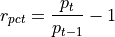
In this case we require the current price and the previous business days price. To do this we can use the lag operator.

@graph
def return_pct(price: TS[float]) -> TS[float]:
    return price / lag(price, 1) - 1.0

The lag operator will delay the release of a value. In this case we are delaying it by one tick, that is when the price is updated, the previous updated value is released. This works really well in backtest where the next price is always available, however, in production or in scenarios where we need to delay a value for say a business day, this does not work. For example, we are computing returns on a schedule, but one of the prices did not tick (say due to a holiday) then we will not compute a return.

Lag also has an option to delay by a specified time, but that does not take into account the difference between days and business days (i.e. the next day could be a weekend), additionally it is very convenient to align the computation to a marker. To assist with this, there is another mechanism to lag the price, namely using the proxy lag option.

This is how we could adjust the computation:

@graph
def return_pct(price: TS[float]) -> TS[float]:
    return price / lag(price, 1, trade_date()) - 1.0

This form of lag uses a proxy time-series to release the lagged value. This will capture the price and after the price was captured the next time the proxy (in this case trade_date()) ticks even if the price does not tick.

The up side of this is that the price is now released on $t-1$ as required for the formula.

For values that were computed we need to make use of the feedback operator. This can be performed in conjunction with the lag operator, but for this example we will consider it without.

For example:

@graph
def compute_index(symbol: TS[str], prices: TSD[str, TS[float]]) -> TS[float]:
    level_fb = feedback(TS[float])
    level = compute_level(prices, prev_level=level_fb())
    level_fb(level)
    return level

This computes the level, which is a path dependant computation, thus requiring the previously computed value to be provided as an input. The feedback makes the value available on the next engine cycle (by default 1 micro-second)

When computing a value using a previous value, it is important to avoid re-computing the value when the feedback ticks on the next engine cycle. This can be achieved in two possible ways, when using value inside of a graph, use the passive marker. This ensures that code the time-series is fed into marks the input as passive. For example:

@graph
def compute_level(prices: TSD[str, TS[float], prev_level: TS[float]) -> TS[float]:
    abs_return = ...
    return abs_return + passive(prev_return)

This will result in a new ticks being generated only when the abs_return ticks.

The other option is when using a compute_node or sink_node, in this case use the active attribute to exclude the input from causing the code to be activated, for example:

@compute_node(active=("prices",))
def compute_level(prices: TSD[str, TS[float], prev_level: TS[float]) -> TS[float]:
    ...

In this case the node will only be evaluated when the prices input is modified.

When this rule is not followed, the graph is likely to go into a tight loop computing values and then feeding them back into the graph. If this were a recursive function we would eventually blow the stack, but since this is not, the graph just cycles and appears to be stuck. This is a classic issue that can be very annoying.

Combining a feedback with a lag is a fantastic way to create better timing alignment for computations, thus using the proxy lag will ensure the the previously computed value is fed into the graph at the next appropriate computation cycle based on the proxy input. Using the previous example, this could look as follows:

@graph
def compute_index(symbol: TS[str], prices: TSD[str, TS[float]]) -> TS[float]:
    level_fb = feedback(TS[float])
    dt = business_day(symbol)
    level = compute_level(prices, prev_level=lag(level_fb(), 1, dt))
    level_fb(level)
    return level

In this approach we do not need to mark the previous value as being passive as it will only tick when the next appropriate computation cycle is started.