Formula and their conversion to HGraph

This section covers examples of common financial formulas and how they can be represented in HGraph.

For the conversion of formulas to HGraph, we use the following definitions:

$t$ is a time-series of TIME_TYPE values, which can be either date or datetime. This is expected to tick with a constant frequency with respect to values being processed. For example when we are pricing this should tick with priceable days. The expected use of this to indicate current value or previous values in the form of:

previous price: $p_{t-1}$
current price: $p_{t}$ .

This works with a lag operator where the $- i$ represents how many ticks of the TIME_TYPE time-series to delay the value by. For example, lag(price, i, t).

Note

This library largely focuses on the simplified view of computations, but the hg_oap library provides more robust solutions to computing prices where dimension units are included with all numbers. This improves the quality of the results as it handles conversions and unit alignment. It is easy to confuse an annual rate with a daily rate when we do not track units in computations, however, tracking units on computations can also add addition expense and complexity. This package is focused on more common patterns followed in the systematic trading community, which tend to make more assumptions of the data (such as pricing in USD, etc.). However, it is possible to apply all the techniques in this library to the price tooling provided by the hg_oap library.

Simple Return

$r_{t} = \frac{p_t}{p_{t-1}} - 1$

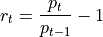
where:

$p_t$ is the price at time $t$
$p_{t-1}$ is the price at time $t-1$ this effectively represents the periodicity of the computation
$r_{t}$ is the return at time $t$

@graph
def simple_return(p: TS[float], t: TS[TIME_TYPE]) -> TS[float]:
    return (p / lag(p, 1, t) - 1.0

Adjusted Returns (for time-period)

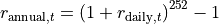
$r_{\text{annual}, t} = \left( 1 + r_{\text{daily}, t}\right)^{252} - 1$

where:

$252$ is the number of periods to convert from the shorter to longer period, in this case the number of trading days in a year.
$r_{\text{daily}, t}$ is the return of the period to be converted at time $t$ , in this case daily.
$r_{\text{annual}, t}$ is the return at time $t$ scaled to the period of interest (in this case annual).

This can be made a bit more generic by using the following formula:

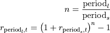
$n = \frac{\text{period}_l}{\text{period}_s} r_{\text{period}_l, t} = \left( 1 + r_{\text{period}_s, t}\right)^{n} - 1$

where:

$n$ is number of periods of the shorter in time to the longer period.
${\text{period}_l}$ is the longer time-period (e.g. annual)
${\text{period}_s}$ is the shorter time-period (e.g. daily)

@graph
def adjusted_return(r: TS[float], n: TS[float]) -> TS[float]:
    return (1.0 + r) ** n - 1.0

This approach also works when converting from a longer period to a shorter period, for example:

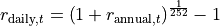
$r_{\text{daily}, t} = \left( 1 + r_{\text{annual}, t}\right)^{\frac{1}{252}} - 1$

where:

$n$ is $\frac{1}{252}$ is the fraction of days in a year.

Excess Returns

This is the comparison of returns vs a risk-free benchmark. This is typically a comparison to a rate such as returns of T-Bills, Overnight Indexed Swap (OIS), etc. Often the Secure Overnight Finance Rate (SOFR) is used as a proxy for a risk-free rate.

$r_{\text{excess}, t} = r_t - r_{f_{t}}$

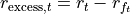
where:

$r_t$ is the return at time $t$
$r_{f_{t}}$ is the risk-free rate at time $t$
$r_{\text{excess}, t}$ is the excess return at time $t$

Note, that the periods of the returns must align.

@graph
def excess_return(r: TS[float], rf: TS[float]) -> TS[float]:
    return r - rf

A more specific example of this may be when using SOFR as the risk-free rate and a daily return as described above, the code may look something like this:

@graph
def my_computation():
    t = business_day("MyInstrument")
    p = price_in_dollars("MyInstrument")
    r_my_inst = simple_return(p, t)
    r_sofr = returns_in_dollars("SOFR")  # This is an annual return
    r_excess = excess_return(r_my_inst, adjusted_return(r_sofr, 1.0/252.0))

Resulting in a daily excess return.

Sharpe Ratio

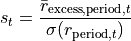
$s_{t} = \frac{\bar{r}_{\text{excess},\text{period},t}}{\sigma(r_{\text{period}, t})}$

where:

$r_{\text{period}, t}$ is the return at time $t$ with the periodicity specified (e.g. daily)
$\bar{r}_{\text{excess},\text{period},t}$ is the mean of the excess return at time $t$ with the periodicity specified.
$\sigma(r_{\text{period}, t})$ is the standard deviation of the returns at time $t$

To compute the volatility ( $\sigma$ ) we need an amount of history. There are a couple of techniques to compute this, but the most common is to use a rolling window. Note, we should align the window with the samples used to compute the mean as well.

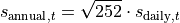
Additionally, the Sharpe ratio is a value in terms of the periodicity of the returns used and may require adjustment to an annual value for comparative purposes.

The adjustment is similar to that used for adjusting returns, however in this case we multiply the ratio by the square root of the number of periods in a year.

$s_{\text{annual}, t} = \sqrt{252} \cdot s_{\text{daily}, t}$

Here is a simple example of the sharpe ratio:

@graph
def sharpe_ratio_annual( r_daily: TS[float], rf_daily: TS[float]) -> TS[float]:
    r_excess = excess_return(r_daily, rf_daily)
    mean_excess_returns = mean(r_excess)
    std_dev_returns = std(r_daily)
    sharpe = mean_excess_returns / std_dev_returns
    return sharpe * math.sqrt(252.0)

or in one-line:

@graph
def sharpe_ratio_annual( r_daily: TS[float], rf_daily: TS[float]) -> TS[float]:
    return mean(excess_return(r_daily, rf_daily)) / std(r_daily) * math.sqrt(252.0)

It is always possible to place the math in a single line of code, but sometimes it is useful to break it up into smaller pieces to make it easier to read and understand, and when debugging, the graph will add additional context information into the generic nodes to help identify the source of a node. The assigned variable is often captured into the meta-data of the node making it easier to trace computations when things go wrong.

Now the version of the code displayed above is a path dependant computation since it uses an expanding window computation. This not often not desirable, instead we may prefer a rolling window which will produce a more stable result.

Here is an example using a rolling window:

@graph
def sharpe_ratio_annual( r_daily: TS[float], rf_daily: TS[float]) -> TS[float]:
    r_excess = to_window(excess_return(r_daily, rf_daily), 252, 30)  # A minimum of 30 samples with a rolling year
    mean_excess_returns = mean(r_excess)
    std_dev_returns = std(to_window(r_daily, 252, 30))  # Apply a uniform window to the std deviation.
    sharpe = mean_excess_returns / std_dev_returns
    return sharpe * math.sqrt(252.0)  # Adjust to make it annualized

The to_window function is a special function that will take the time-series and convert it into a widowed value. This is capable of supporting time as well as an integer count based windows. However, time time-based window is not capable of understanding the concept of business days, etc. so the windows are always exact time durations. In the world of systematic trading that is not the most useful approach, so using the count and aligning the input to events such as business days is more useful as a rule.